Speedrunning and Speedcubing: Eerily Similar and Surprisingly Different

You’ve probably been frustrated trying to play a video game. You’ve also probably been frustrated trying to solve a Rubik’s Cube. These frustrations can be quite similar. But what about doing both super fast?

If you’ve been reading my posts, you know I’ve talked about speedrunning before, specifically the history of the any% speedrun of the 1985 video game Super Mario Bros.

To refresh, a speedrun is a playthrough of a video game to satisfy an objective in the fastest time possible. Speedrunning has become much more than a hobby over the past decade, with events such as Games Done Quick and websites like Twitch to help popularize it. Any full recorded attempt that is done in the quickest time possible will be eligible for World Record (or WR for short) status, with speedrun.com functioning as the main body for verifying runs. The aforementioned website also acts as an archive for previous runs as well as a place for other speedrunners to submit their own personal bests (or PB for short).

Now, you might be wondering… what does speedrunning have to do with speedcubing? And what even IS speedcubing? Well…

Speedcubing refers specifically to solving a combination puzzle, most famously the Rubik’s Cube, in the fastest time possible. Unlike with speedrunning, where any personal best can be submitted for a world record, the World Cubing Association (WCA) only accepts attempts done at official competitions, a major difference between the two. This aspect I will discuss later, so let us discuss how speedcubing became a thing, where it is now, and where it can go, all while drawing parallels to speedrunning. Additionally, we will focus strictly on the 3x3x3 Rubik’s Cube, as other cubes of other sizes have their own histories.

Chapter 1: Genesis of the Rubik’s Cube

In 1970, Larry D. Nichols invented a 2x2x2 “puzzle with pieces rotatable in groups” held together by magnets, the predecessor to the modern Pocket Cube, the 2x2x2 variant of the Rubik’s Cube.

In the mid-1970s, Ernő Rubik, then part of the Department of Interior Design at the Academy of Applied Arts and Crafts in Budapest, sought to create a structure of cubes that could rotate independently but without the entire thing falling apart. Upon successfully creating such a structure, he had inadvertently created the puzzle that became known as the Rubik’s Cube, as the more he twisted, the colors became more scrambled, and he was unsure if this new problem could be solved. He would later show this to his students, leading to the misconception that he had invented the puzzle for his students as a teaching tool to understand 3D objects. Rubik would eventually apply for a patent for his “Magic Cube” on January 30, 1975, which would be granted later that year.

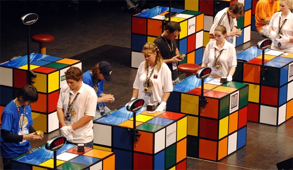
By the early 1980s, the puzzle took the world by storm. On June 5th, 1982, 19 of the fastest solvers gathered for the first ever Rubik’s Cube World Championship, where Rubik himself was a delegate. The fastest time at the competition was 22.95 seconds by Minh Thai of the United States, the first ever World Record. Eventually, the puzzle would fade in popularity, and no competitions were held for over two decades.

Despite this, it was during these first several years that methods to solving the cube developed. One such method is the Petrus method, developed by Lars Petrus of Sweden, which involves strong intuition and “block-building” and is popular for solving the cube in the fewest moves (it is also the method that I use as a casual solver). Petrus himself finished fourth overall in the competition in 1980. However, this method has largely faded amongst speedcubers in the modern day due to the predominance and efficiency of other methods, including one known as CFOP.

CFOP stands for Cross-F2L-OLL-PLL, where F2L stands for “First 2 Layers“, OLL stands for “Orient Last Layer“, and PLL stands for “Permute Last Layer“. This method is built upon the idea layer-building, where solvers must solve the cube one layer at a time, and layer-building has been a loose method that has been in use since the earliest days of the puzzle. CFOP stands over beginner methods in a multitude of ways: the F2L step solves two layers at once, while OLL and PLL can be completed with one algorithm each. Wait… what is an algorithm in the Rubik’s Cube sense?

Whereas “algorithm” usually means “a set of rules to be followed in calculations”, the term in a Rubik’s Cube sense refers to “a set of moves used to orient the cube a certain way“. The universal notation is noted above, where letters are used to let solvers know of which layer or face to turn. Any letter on its own tells the solver to turn its associated face clockwise as if they were looking directly at it. If the solver needs to turn the face counter-clockwise, a prime symbol (‘) is affixed to the letter, similar to how it is used in mathematics to denote the complement (or “opposite”) of a set (sometimes a lower case “i” is used for “inverted”, although this is generally frowned upon because lower case letters are used for more advanced notation). Turning a layer twice leads to a “2” being suffixed to a letter (ex “R2” tells a solver to turn the “Right” layer twice).

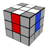
In essence, algorithms are used to manipulate the Rubik’s Cube into a favorable situation, as they are used to get to a certain scenario. To best illustrate this, let us discuss in essence how the beginner’s version of CFOP works, sometimes referred to as the “Dan Brown” method after the eponymous former vlogger who popularized it on YouTube (and an equally in-depth guide can be found here, and I will be sourcing some images from this website for this chapter): First, solvers must form a cross on one side in a way that the edge pieces of the cross are correctly placed. How anyone can know this is because the center pieces of every Rubik’s Cube are fixed and do not move, meaning everyone will know which layer correspond to which color. For simplicity, most beginners usually start by staying with one color for the cross when practicing (usually white or green). This step is largely intuitive, and while some of the moves are largely identical such that algorithms can technically be transcribed, they usually aren’t for simplicity.

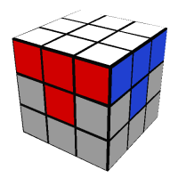
Upon forming the cross, solvers need to place the corners of the layer with the cross into position without breaking the cross. This step has numerous names for beginner’s context, either “The Corners” or “Solve First Layer” or “F2L1”. In this step, the first major algorithm appears, and it’s used to position the corners correctly. Additionally, the algorithm might be performed multiple times.

The next step (sometimes referred to as “Solve Second Layer” or “F2L2”) involves placing the four edges in the middle layer (or second layer) in place without breaking the first layer. By this point, the solved layer becomes the bottom or “Down” face (D). Again, algorithms are taught to beginners here to place the edge pieces properly.

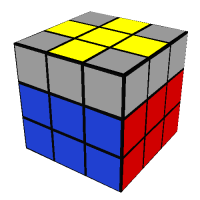
From this point forward, every step involves the last layer and solving it without sacrificing the previous two in the process. The first part involves getting a cross on the last year much like the first one, although it does not necessarily need to be oriented as properly like the first. Upon finishing the previous step, there will be four different scenarios. Should a cross already appear, this step is skipped, but the other three scenarios involve using one of two algorithms (one case requires both) to achieve a cross.

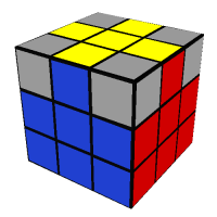
The next step involves actually getting the cross oriented correctly much like the first step, and the algorithm used here effectively “swaps” the positions of two adjacent edges.

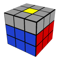
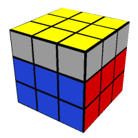
Afterwards, solvers need to get the corners in the correct place, and the algorithm used swaps the position of three corners in a counter-clockwise-fashion. How solvers can verify if corners are in the correct position is by using the centers as reference. For example…

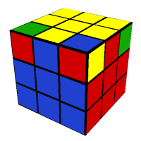
In the above image, the corner with red, blue, and yellow is in its correct position (albeit not oriented or permuted properly), while the other three are not, meaning the algorithm is used to swap the positions of the other three corners.

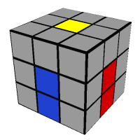
Upon getting the corners to the correct positions, the last step requires getting the corners to be oriented/permuted properly, and the algorithm used is actually the same as the one to position the corners following the first cross. Upon the orienting/permuting the final corner, the cube will be solved!

Now why this long explanation of how to solve the cube? Well as mentioned before, CFOP shortens the previous steps significantly. First off, the cross is formed on the bottom as turning the cube as a whole wastes time. Secondly, F2L in CFOP immediately follows the cross and seeks to place both the corners and edges into their positions simultaneously as opposed to placing first the corners and then the edges. Then comes the magic.

Upon finishing F2L, there are 57 total cases that the cube will be in, and there exists at least one algorithm to get the cube to have the final face into one color for each case, a step, as mentioned before, known as OLL (if the final face is already one color after finishing F2L, you’ve technically arrived at Case 58 in which you proceed directly to the next step). There are then 21 cases the cube will be in following OLL (the “solved” case is an unofficial 22nd case and is rather uncommon after finishing OLL), and just like before, there is at least one algorithm for each case to solve the cube; the step known as PLL. The fact that upon finishing F2L, that only two algorithms separate a solver from finishing should go to show just how fast CFOP is. The initial algorithms for OLL and PLL were developed by Jessica Fridrich of Czechia, which is why CFOP is sometimes referred to as the Fridrich method.

Chapter 2: Genesis of Speedcubing

It wasn’t until 2003 when the World Cube Association (WCA) was founded by various online enthusiasts that kept the interest of speedcubing alive. Wishing to meet in person and compete, from August 23 to 24 in 2003, the WCA held the first competition in over two decades. Dan Knights of the United States broke the 20-second barrier with a time of 16.71, then Jess Bonde of Denmark broke it at the same competition with a time of 16.53. In 2004, Shotaro Makisumi of Japan shattered the record further with a time of 12.11. The record then went further down as time went on over the next few years. Here’s a timeline through February 24, 2007:

Date	Contestant	Citizenship	Event	Time
June 5, 1982	Minh Thai	United States	World Rubik’s Cube Championship 1982	22.95
August 23, 2003	Dan Knights	United States	World Rubik’s Cube Championship 2003	16.71
August 23, 2003	Jess Bonde	United States	World Rubik’s Cube Championship 2003	16.53
January 24, 2004	Shotaro Makisumi	Japan	Caltech Winter Competition 2004	15.07
January 24, 2004	Shotaro Makisumi	Japan	Caltech Winter Competition 2004	14.76
April 3, 2004	Shotaro Makisumi	Japan	Caltech Spring Competition 2004	13.93
April 3, 2004	Shotaro Makisumi	Japan	Caltech Spring Competition 2004	12.11
October 16, 2005	Jean Pons	France	Dutch Open 2005	11.75
January 14, 2006	Leyan Lo	United States	Caltech Winter Competition 2006	11.13
August 4, 2006	Toby Mao	United States	US Nationals 2006	10.48
February 24, 2007	Edouard Chambon	France	Belgian Open 2007	10.36

Before we continue, consider the fact that it was also during the mid-2000s that achieving high scores in video games and speedrunning regained interest amongst some of the general public. Yet another parallel between speedcubing and speedrunning: not only are their internal concepts similar, but their own histories and genesis were also similar.

Anyway, the first to solve a Rubik’s Cube under 10 seconds was Thibault Jacquinot of France, doing so with 9.86 seconds at the Spanish Open 2007 on May 5. Some believed that this would stand for a long time with this monumental feat, but Erik Akkersdijk of the Netherlands broke it at the Dutch Open five months later with a time of 9.77 seconds. Ron van Bruchem, one of the founders of the WCA, broke that about a month and a half later at the Dutch Championship with a time of 9.55. Chambon would take it back at the Murcia Open the following year with a time of 9.18. However…

Yu Nakajima broke the 9-second barrier with a time of 8.72 at the Kashiwa Open on May 5, exactly a year after Jacquinot broke the 10-second barrier. What made his feat so remarkable was that he achieved the same time TWICE, the second being in the final of the event.

However, this only stood for about three months.

In what many considered the greatest record at the time, Erik Akkersdijk yanked it back by shaving off over a second and a half with a final time of 7.08. This record became widely publicized and it stood for a remarkable 854 days. Until it was broken, this was the longest standing record since Minh Thai’s from 1982.

Chapter 3: Speedcubing takes off

If you recall anything about the Super Mario Bros any% speedrun, it’s that there were numerous moments when the category was thought to be dead. Indeed, Erik Akkersdijk’s 7.08 nearly represented a point when the World Record was just going to end there. However, as you can recall, practice runs do not count towards World Records, but they can show how fast they can be. The previous video I had shown on Yu Nakajima was a practice solve with a time of 6.57, which was technically FASTER than the record of 7.08. So if it was possible to do in practice, could it be done in competition?

By 2010, Feliks Zemdegs, a young speedcuber from Australia, was beginning his meteoric rise. He had set the World Record for an average of five solves on January 30, 2010 at 9.21 at the Melbourne Summer Open 2010, and in just over nine months, he broke the record for a single solve with 7.03 seconds at Melbourne Cube Day 2010. However, he wasn’t done that day: he broke the 7-second barrier in the same competition with a time of 6.77.

One of Feliks’s major advantages was his color neutrality, a strategy that dates as early as Lars Petrus in the 1980s, who used his method WITH color neutrality to reach the championship in 1982. This concept revolves around being able to solve the cube from any point and with little regard to starting color. Previously with CFOP, speedcubers would fix to one color for the cross (meaning they always made a cross of the same color) as it gave better results when beginning for F2L, as every speedcuber is given an inspection time to analyze where the pieces they need are and to plan their solve ahead of time. Indeed, prior to 2007, no CFOP user recommended color neutrality as a viable strategy. However, even casual solvers such as Dan Brown had recommended color neutrality as a way to solve faster. Indeed, Rowe Hessler’s success in 2008 is attributed to color neutrality, and then it was Feliks who propelled it even further.

Throughout 2011, Feliks proceeded to take his own records further. By the end of the year, 6.77 felt like nothing.

Date	Date	Time
January 29, 2011	Melbourne Summer Open 2011	6.65
May 7, 2011	Kubaroo Open 2011	6.65
May 7, 2011	Kubaroo Open 2011	6.24
June 25, 2011	Melbourne Winter Open 2011	6.18
June 25, 2011	Melbourne Winter Open 2011	5.66

By the middle of 2011, Feliks had switched to using a cube manufactured by DaYan, a Chinese cube maker and one of many from China that had begun making cubes optimized for speedsolves (more of these companies have popped up since, including GAN, who now sponsor Feliks). Additionally, his 5.66 was another second-shattering record and one that again stood unmatched for nearly two years.

On March 2, 2013, Dutch speedcuber Mats Valk took the record with a time of 5.55 seconds. This one would stand for over two years. Then American speedcuber Collin Burns would take the record on April 25, 2015 at the Doylestown Spring 2015 with a time of 5.25 seconds. As remarkable as these breakthroughs were, something bigger was on the horizon.

On November 21, 2015 at the River Hill Fall 2015, Collin Burns managed a 5.21 on a bad scramble from the officials, then Keaton Ellis managed a 5.09 at the same competition. However, it was Lucas Etter who wound up in the books, shattering both times with a 4.90, the first ever solve in competition under 5 seconds. A new world record.

Afterwards, numerous speedcubers took the record in an all-out blitz over the next few years, and there were some familiar faces who took it back…

Date	Contestant	Citizenship	Event	Time
November 5, 2016	Mats Valk	Netherlands	Jawa Timur Open 2016	4.74
December 11, 2016	Feliks Zemdegs	Australia	POPS Open 2016	4.73
September 2, 2017	Patrick Ponce	United States	Rally In The Valley 2017	4.69
October 28, 2017	SeungBeom Cho	South Korea	ChicaGhosts 2017	4.59
January 27, 2018	Feliks Zemdegs	Australia	Hobart Summer 2018	4.59
May 6, 2018	Feliks Zemdegs	Australia	Cube for Cambodia 2018	4.22

Feliks’s 4.22 is his latest world record, as someone else bested him on November 24 that year…

Yusheng Du of China kind of just broke it open. His remarkable 3.47 remains the current world record. The four-second barrier had been broken. This solve was slightly controversial as the footage was only caught on a security camera at a rather awkward angle, but it has been analyzed and confirmed by numerous people in the community, including Phillip Lewicki and prominent YouTuber and speedcuber Dylan Wang (better known as J Perm). Regardless, this time has stood for an astonishing three years, longer than any previous record outside the first one by Minh Thai nearly 40 years ago.

Chapter 4: Future of the 3x3x3

You might be wondering once more if this time has even been bested or even come close in practice. The answer is YES, multiple times. In fact, there have been solves in practice under three seconds (THREE!!!). However, there had been some skepticism in the first several months over whether it was even possible following the new world record.

This is where I present to you some of the remarkable feats that speedcubers have accomplished since in practice, some of which include analyses:

Solving the 3x3x3 under four seconds, once considered a pipe-dream, has now been done numerous times in practice. There are also now at least four to have solved it in under three seconds (THREE!!!) in practice: Max Park, Fahmi Aulia Rachman, Leo Borromeo, and Ruihang Xu. Fahmi Aulia Rachman happens to hold the fastest in practice with a time of 2.62 (reconstruction here), and he did so using a rather uncommon but notable method for speedcubing known as the Roux method (named after its French founder Gilles Roux).

Regardless, it seems obvious that a time under three seconds can THEORETICALLY be achieved in competition given that personal bests have been achieved in practice, however, there are many factors that weigh against this. While many can attribute the remarkable advances in speedcubing to tricks and strategy, what can separate a good solve from a bad solve involves an infamous metric that can NEVER be quantified: luck.

Consider luck the speedcubing equivalent or parallel to RNG in speedrunning. Good RNG in a speedrun can keep a good speedrun alive as it does with “hands” in Super Mario Bros. 3 (a good explanation of what this means can be found here), while bad RNG can absolutely sink it. This can happen in speedcubing: a lucky solve can result in a skip in steps or just simple ease in the process of solving, and this can be potentially exploited during the inspection phase, as seen in Leo Borrameo’s 3.57 (his surprise exemplifies this).

Consider the fact that thus far, we have largely been discussing a single solve. As mentioned in the video by Wired, most speedcubers don’t even care much for the single solve, instead taking great care in the World Record average, which as mentioned before, is taken with an average of five solves (in reality, the best and worst times of the five are not considered and the remaining three are then averaged). Speedcubers consider the average a true test of skill. Even if you get a lucky solve, your average will reflect just how quickly you can usually solve the cube. Feliks himself has set the World Record for average more than anyone else, and his best average of 5.53 was the WR from November 10, 2019 (when he set it at Odd Day in Sydney 2019) until Ruihang Xu beat it at the Wuhan Open 2021 with an average of 5.48. Max Park of the United States broke this about five months later with an average of 5.32, then it was Tymon Kolasiński of Poland who took it down further at Cubers Eve Lubartów 2021 with an average of 5.09.

These are where the records stand today. Who will beat Yusheng Du in competition? Will someone average better than Tymon? Can anyone average under five seconds? Might I oblige with a statement from speedrunning, specifically the golden rule: the limits are never where we think they are.